Research / Statistical arbitrage
Walk-forward cointegration pairs trading, with a placebo and multiple-testing control
Abstract. I test whether cointegration-selected pairs of US large caps earn anything out of sample, on 102 stocks over 40 walk-forward windows from January 2007 to November 2026. After costs the answer is no. Of 20,040 pair-window cointegration tests, 6.6% pass at the 5% level (pure noise would give at most 5%) and only 86 survive false-discovery control, in 12 of the 40 windows. Trading those survivors gives a net Sharpe ratio of 0.16 (95% bootstrap interval -0.25 to 0.65); the conventional uncorrected p < 0.05 selection gives 0.12 (-0.37 to 0.58), which is the 83rd percentile of 1,000 portfolios of random within-sector pairs traded with the same rule (one-sided p = 0.17), and its net Sharpe falls from 0.69 in 2007-2012 to -0.78 in 2020-2026. The simpler distance method of Gatev, Goetzmann and Rouwenhorst does better at 0.41 (0.04 to 0.79), and selected pairs pass the cointegration test again in the trading window about 8% of the time against 7% for an arbitrary pair.
- Question
- Do cointegration-selected pairs earn anything out of sample, after costs, beyond what random pairs earn?
- Data
- 102 US large caps, daily adjusted closes, 40 walk-forward windows from January 2007 to November 2026
- Methods
- Engle-Granger cointegration, Benjamini-Hochberg false-discovery control, Ornstein-Uhlenbeck maximum likelihood, stationary bootstrap, random-pair placebo, deflated Sharpe ratio
- Verification
- 36 tests, including no-look-ahead checks on selection and signals, and hand-computed P&L with costs and execution lag
The question
Pairs trading is the standard first statistical-arbitrage strategy: find two stocks whose prices move together, wait for the spread to open, bet on it closing. It is also a strategy where a backtest can mislead in many ways at once. Hundreds of pairs are tested per period, so some look cointegrated by chance. Hedge ratios and thresholds are easy to fit with data from the period being traded. Costs are of the same order as the edge. And a contrarian rule applied to any pair of similar stocks may earn something without the selection step adding anything.
So the question here is narrow: does a formal cointegration test, applied honestly, pick pairs that mean-revert in the following six months, after costs, by more than random pairs from the same sector do? I fixed the design before computing any returns and report what came out.
The mathematics
Cointegration (Engle and Granger, 1987). Two log-price series \(y_t\), \(x_t\) that are each integrated of order one are cointegrated if some \(\beta\) makes \(y_t - \beta x_t\) stationary. The two-step test is
$$y_t = \alpha + \beta x_t + e_t \quad\text{(OLS)}, \qquad \Delta \hat e_t = \rho\, \hat e_{t-1} + \gamma\, \Delta \hat e_{t-1} + u_t ,$$and the statistic is the \(t\)-ratio of \(\hat\rho\). Deterministic terms: a constant in the cointegrating regression, none in the residual regression, one lagged difference. Because \(\hat e_t\) is a fitted residual the statistic does not follow the Dickey-Fuller distribution; I use MacKinnon's response-surface p-values for two series with a constant. The test is not symmetric in \(y\) and \(x\), so I run both directions, keep the one with the more negative statistic and double its p-value (a Bonferroni correction over the two directions). stats.engle_granger is my own implementation and is tested to agree with statsmodels.tsa.stattools.coint to eight digits.
False discovery rate (Benjamini and Hochberg, 1995). With \(m = 501\) pairs tested per window, sort the p-values \(p_{(1)} \le \dots \le p_{(m)}\), find
$$k = \max\{\, i : p_{(i)} \le i\,q/m \,\},$$and reject the \(k\) smallest. This bounds the expected share of false discoveries among the rejections by \(q\) when the tests are independent or positively dependent. I use \(q = 0.10\).
Ornstein-Uhlenbeck spread. I model the spread \(X_t = y_t - \beta x_t\) as
$$dX_t = \kappa(\mu - X_t)\,dt + \sigma\,dW_t .$$Applying Itô's lemma to \(e^{\kappa t}X_t\) and integrating over a step \(\Delta\) gives the exact transition
$$X_{t+\Delta} = \mu + (X_t - \mu)\,e^{-\kappa\Delta} + \varepsilon_t, \qquad \varepsilon_t \sim N\!\left(0,\ \sigma^2\,\frac{1 - e^{-2\kappa\Delta}}{2\kappa}\right),$$which is an AR(1), \(X_{t+\Delta} = a + b X_t + \varepsilon_t\), with \(b = e^{-\kappa\Delta}\) and \(a = \mu(1-b)\). The conditional Gaussian likelihood is maximised by least squares, \(\hat b = \widehat{\mathrm{Cov}}(X_t, X_{t+\Delta}) / \widehat{\mathrm{Var}}(X_t)\), \(\hat a = \bar X_{+} - \hat b \bar X\), \(\hat\sigma_\varepsilon^2 = \tfrac1n \sum \hat\varepsilon_t^2\), and inverting the map gives
$$\hat\kappa = -\frac{\ln \hat b}{\Delta}, \qquad \hat\mu = \frac{\hat a}{1 - \hat b}, \qquad \hat\sigma^2 = \hat\sigma_\varepsilon^2\,\frac{2\hat\kappa}{1 - \hat b^2} .$$Since \(E[X_{t+h} - \mu \mid X_t] = (X_t - \mu)e^{-\kappa h}\), a deviation halves in \(h_{1/2} = \ln 2/\kappa\). stats.ou_mle implements this.
Signal and P&L. With \(\mu_S\), \(\sigma_S\) the formation-window mean and standard deviation of the spread, the out-of-sample z-score is \(z_t = (y_t - \beta x_t - \mu_S)/\sigma_S\). A position is one dollar long one leg and one dollar short the other, so its return is approximately
$$r_{y,t} - r_{x,t} \;\approx\; \Delta S_t + (\beta - 1)\,\Delta \log P_{x,t}.$$The first term is the spread the signal is about; the second is unhedged exposure to \(x\) whenever \(\beta \ne 1\). I return to this below because it matters.
Sampling error of a Sharpe ratio. I report three things. (i) A percentile interval from the stationary bootstrap of Politis and Romano (1994), mean block 21 days, 2,000 resamples. (ii) Lo's (2002) standard error for serially correlated returns: with \(g(\mu, \sigma^2) = \mu/\sigma\) and \(\Sigma\) the Newey-West long-run covariance of the moment conditions \((r_t - \mu,\ (r_t-\mu)^2 - \sigma^2)\),
$$\mathrm{Var}(\widehat{SR}) = \frac{1}{T}\,\nabla g^\top \Sigma\, \nabla g, \qquad \nabla g = \left(\frac1\sigma,\ -\frac{\mu}{2\sigma^3}\right),$$which reduces to \((1 + SR^2/2)/T\) for i.i.d. normal returns. (iii) The deflated Sharpe ratio of Bailey and López de Prado (2014) for a result picked from \(N\) trials:
$$SR_0 = \sqrt{V}\left[(1-\gamma)\,\Phi^{-1}\!\left(1 - \tfrac1N\right) + \gamma\,\Phi^{-1}\!\left(1 - \tfrac{1}{Ne}\right)\right], \qquad DSR = \Phi\!\left(\frac{(\widehat{SR} - SR_0)\sqrt{T-1}}{\sqrt{1 - \gamma_3 \widehat{SR} + \frac{\gamma_4 - 1}{4}\widehat{SR}^2}}\right),$$with \(V\) the variance of the Sharpe estimates across trials, \(\gamma\) Euler's constant, and \(\gamma_3\), \(\gamma_4\) the skewness and kurtosis of returns.
Method
Everything in this section was fixed before any return was computed, with one exception that I flag.
Data. Daily closes adjusted for splits and dividends from Yahoo Finance, 3 January 2005 to 13 November 2026 (5,502 days). The universe starts from the S&P 100 as listed in September 2026, minus Alphabet's second share class, plus 19 large S&P 500 names in the four sectors (Energy, Utilities, Materials, Real Estate) where the S&P 100 has at most three stocks with a full history. Dropping every ticker without a complete history from January 2005 leaves 102 stocks in 11 GICS sectors and 501 within-sector pairs.
Walk-forward. Formation window of 504 trading days, then 126 days of trading, rolled forward 126 days: 40 windows, the first trading day being 4 January 2007 and the last window 84 days long. The hedge ratio, spread mean and standard deviation, OU parameters and the selection itself use formation data only.
Selection. Engle-Granger on log prices for all 501 pairs; Benjamini-Hochberg at \(q = 0.10\) across the 501; then \(\beta > 0\) and an OU half-life between 5 and 60 days; then the 20 most negative test statistics, taking pairs greedily so that no stock sits in more than two.
Trading rule. Short the spread when \(2 \le z < 4\), long when \(-4 < z \le -2\). Close when \(z\) returns to 0. If \(|z|\) reaches 4, close and retire the pair for the rest of the window. Everything is closed at the last close of the window. A decision made on the close of day \(t\) is filled at the close of day \(t+1\).
Costs. 5 bp of traded notional per leg per one-way trade, and 50 bp per year on the value of the short leg.
Capital convention. The portfolio has 20 equal slots. A selected pair occupies one slot; when open it holds \$1 long and \$1 short per \$1 of slot capital, with share counts fixed until the close-out. Empty slots and flat pairs earn nothing. The daily portfolio return is the sum of pair P&L divided by 20. Returns are treated as excess returns; no interest is credited on idle capital.
Comparisons.
- Distance method (Gatev et al., 2006): the 20 within-sector pairs with the smallest sum of squared differences between normalised prices in formation, traded with the identical rule on the z-score of the normalised price difference.
- Placebo: 1,000 draws (seed fixed). Each draw picks, in every window, as many pairs as the strategy held, uniformly at random from within-sector pairs with \(\beta > 0\), under the same per-stock cap, and trades them with the same rule, parameters estimated the same way, and the same costs. The only thing removed is the statistical selection.
- SPY buy and hold, for context.
The exception. The false-discovery-controlled strategy is the design I started with. Once I had the formation tables, and before computing any returns, the discovery counts showed that it would be in cash most of the time. I therefore added a second arm that uses the conventional uncorrected rule p < 0.05 with everything else unchanged. Both arms are reported in full. The second is what most pairs-trading write-ups do, and it is the arm with enough trades to say anything about decay.
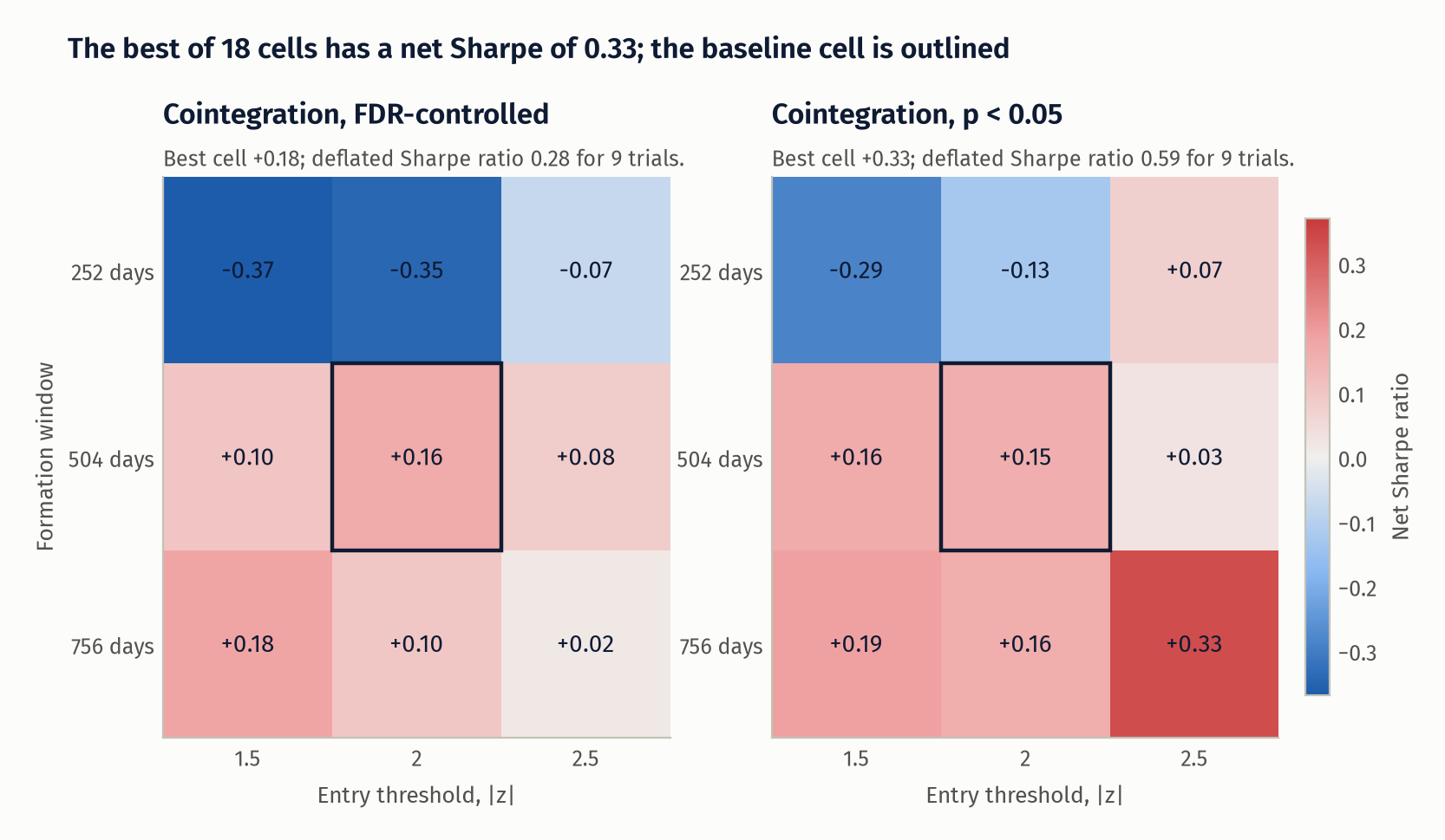
Sensitivity. Entry threshold {1.5, 2.0, 2.5} by formation length {252, 504, 756}, nine cells per arm, all on the same trading calendar from January 2008. I ran this after the baseline and did not change the baseline.
Tests. 36 tests cover: OU parameter recovery on simulated paths over five seeds; Benjamini-Hochberg against the worked example of the 1995 paper; my Engle-Granger against statsmodels, plus its size on independent random walks; the state machine on a scripted path; pair P&L against hand-computed numbers including costs and the one-day lag; that perturbing prices after day \(t\) leaves all portfolio returns up to \(t\) bit-identical and that perturbing the trading window leaves selection unchanged; that independent random walks give a gross Sharpe indistinguishable from zero; Lo's standard error against its i.i.d. closed form; and the deflated Sharpe ratio against the numerical example in Bailey and López de Prado.
Results
Almost nothing survives multiple-testing control, and what does is not persistent
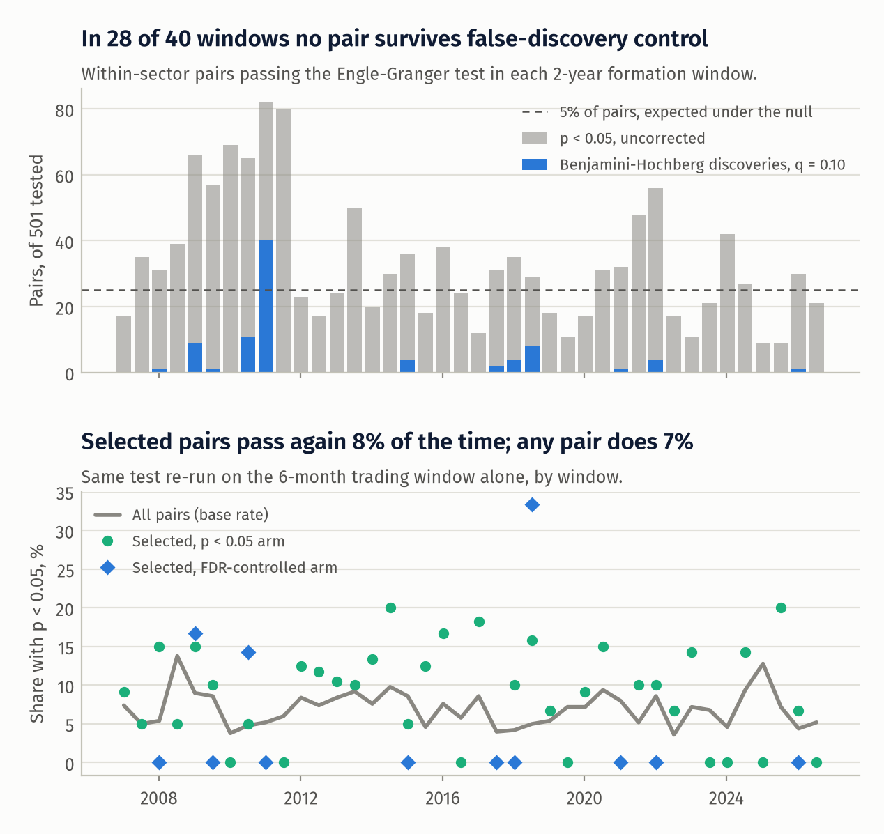
Top: 6.6% of the 20,040 pair-window tests have \(p < 0.05\), against 5% under the null of no cointegration anywhere. Benjamini-Hochberg leaves 86 discoveries in total, and none at all in 28 of 40 windows. Bottom: re-running the test on the trading window alone, pairs selected by the FDR-controlled arm pass 6% of the time, pairs from the p < 0.05 arm 8%, distance pairs 8%, and all 501 pairs 7%. A six-month test has little power, so this does not prove the relationships vanish, but selected pairs are indistinguishable from unselected ones on this measure.
A second sign of overfitting in formation: the median OU half-life of selected pairs is 8.4 days (FDR arm) and 11.6 days (p < 0.05 arm), yet the average round trip lasts 42 and 40 days. Picking the most negative test statistics picks the most overestimated mean-reversion speeds.
Performance, January 2007 to November 2026
| Cointegration, FDR-controlled | Cointegration, p < 0.05 | Distance method | |
|---|---|---|---|
| Annualised return, gross | +0.24% | +0.94% | +2.12% |
| Annualised return, net | +0.20% | +0.45% | +1.52% |
| Annualised volatility, net | 1.25% | 3.66% | 3.67% |
| Sharpe ratio, gross | +0.19 | +0.26 | +0.58 |
| Sharpe ratio, net | +0.16 | +0.12 | +0.41 |
| 95% bootstrap interval | [-0.25, +0.65] | [-0.37, +0.58] | [+0.04, +0.79] |
| Lo (2002) standard error | 0.24 | 0.24 | 0.19 |
| Maximum drawdown, net | -4.7% | -22.8% | -8.4% |
| Beta to SPY | +0.003 | +0.016 | +0.028 |
| Alpha, annualised | +0.17% | +0.28% | +1.22% |
| Alpha t-statistic (Newey-West) | +0.58 | +0.33 | +1.71 |
| Round trips | 52 | 678 | 791 |
| Hit rate, net | 50.0% | 47.6% | 48.9% |
| Average holding period, days | 42.0 | 39.8 | 49.5 |
| Average net P&L per round trip, bp of pair capital | +153 | +27 | +76 |
| Turnover, traded notional per unit capital per year | 0.53 | 6.92 | 8.07 |
| Average pairs selected (of 20 slots) | 1.4 | 16.3 | 20.0 |
| Average gross exposure | 0.04 | 0.54 | 0.78 |
Returns are per unit of committed capital, and most of that capital is idle: the FDR arm fills 1.4 of 20 slots on average, which is why its return and volatility are so small. The Sharpe ratio does not depend on that scaling. Neither cointegration arm has a Sharpe interval that excludes zero or an alpha t-statistic above 0.6. The distance method's interval just excludes zero, with an alpha t-statistic of 1.71. Market betas are all below 0.03. For context, SPY over the same dates had an excess return of 10.6% a year, a Sharpe ratio of 0.54 and a maximum drawdown of -56%.
Against random pairs
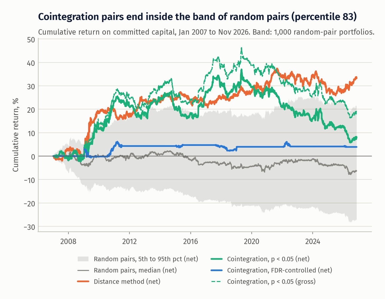
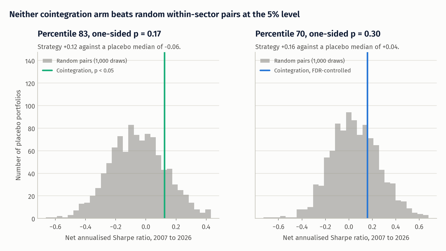
The placebo matched to the p < 0.05 arm has a median net Sharpe of -0.06 (5th to 95th percentile -0.36 to +0.26). The strategy's 0.12 is its 83rd percentile, a one-sided p-value of 0.17. For the FDR arm the placebo median is +0.04 (-0.27 to +0.40) and the strategy's 0.16 is the 70th percentile, p = 0.30. Random within-sector pairs roughly break even before costs (median gross Sharpe +0.04) and lose a little after. The cointegration filter is not distinguishable from picking pairs at random.
Decay
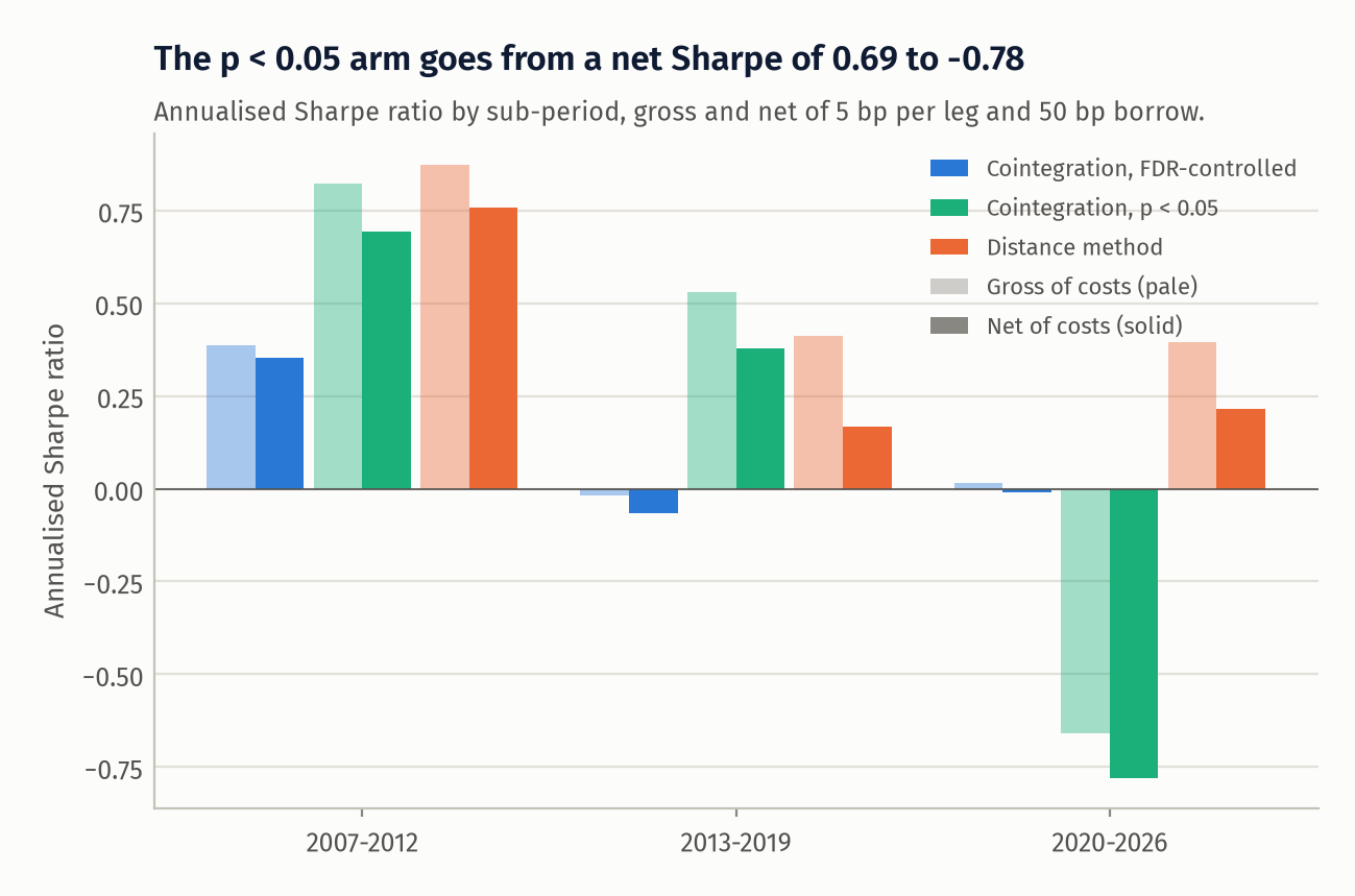
| Net Sharpe (gross) | 2007-2012 | 2013-2019 | 2020-2026 |
|---|---|---|---|
| Cointegration, FDR-controlled | +0.35 (+0.39) | -0.07 (-0.02) | -0.01 (+0.01) |
| Cointegration, p < 0.05 | +0.69 (+0.82) | +0.38 (+0.53) | -0.78 (-0.66) |
| Distance method | +0.76 (+0.87) | +0.17 (+0.41) | +0.22 (+0.40) |
| Placebo percentile of cointegration, p < 0.05 | 98 | 95 | 1 |
| Placebo percentile of cointegration, FDR-controlled | 68 | 51 | 55 |
The p < 0.05 arm beat 98% and 95% of random-pair portfolios in the first two sub-periods and lost to 99% of them in the third. With three sub-periods and a full-sample result that is not significant, I read this as weak evidence of an edge that existed and decayed, in line with Do and Faff (2010), and not as two wins and a loss. The 2007-2012 number is also the one most exposed to survivorship bias (see below). Costs take 0.12 to 0.24 off the Sharpe ratio of the two fully invested arms in every sub-period; the 2020-2026 loss is negative before costs.
One pair, as traded
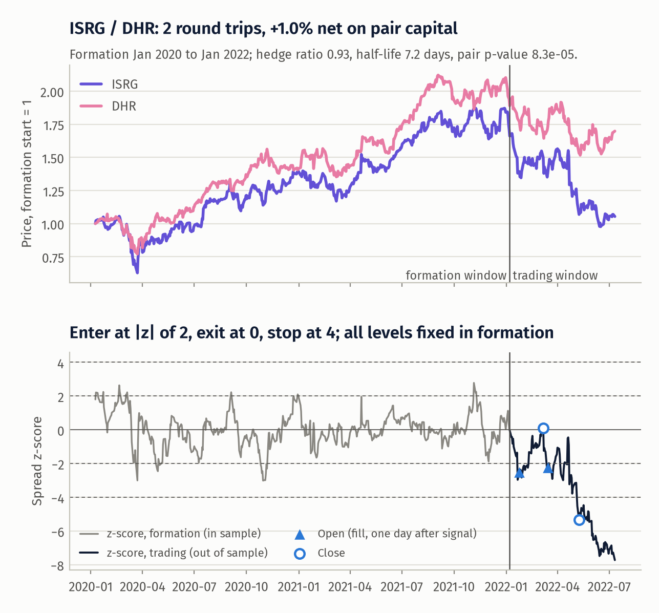
ISRG against DHR in the window starting 7 January 2022 (hedge ratio 0.93, formation half-life 7.2 days, pair p-value 8.3e-05). I chose it by rule: among FDR-arm pair-windows with at least two round trips, the one with the median net P&L. The first trade converges; the second is stopped out as the spread runs through \(|z| = 4\) and keeps going. Net +1.0% on pair capital. The spread that looked stationary for two years stopped being so within a few months, which is the bottom panel of the first figure in one picture.
Sensitivity, in full
| Cointegration, FDR-controlled: net Sharpe | entry 1.5 | entry 2 | entry 2.5 |
|---|---|---|---|
| formation 252 days | -0.37 | -0.35 | -0.07 |
| formation 504 days | +0.10 | +0.16 | +0.08 |
| formation 756 days | +0.18 | +0.10 | +0.02 |
| Cointegration, p < 0.05: net Sharpe | entry 1.5 | entry 2 | entry 2.5 |
|---|---|---|---|
| formation 252 days | -0.29 | -0.13 | +0.07 |
| formation 504 days | +0.16 | +0.15 | +0.03 |
| formation 756 days | +0.19 | +0.16 | +0.33 |
Sample: January 2008 onward, so the baseline cells differ slightly from the headline numbers. Net Sharpe ranges from -0.37 to +0.18 for the FDR arm and from -0.29 to +0.33 for the p < 0.05 arm. One-year formation windows are worse throughout. The best p < 0.05 cell (756 days, entry 2.5) has a Sharpe of 0.33, but the expected maximum of nine zero-skill trials with this dispersion is 0.28, and its deflated Sharpe ratio is 0.59. For the FDR arm the best cell is 0.18 against an expected maximum of 0.31, a deflated Sharpe ratio of 0.28. Nothing in the grid comes near the 0.95 one would want. Using \(N = 9\) treats correlated cells as independent, which overstates the deflation somewhat; the conclusion does not depend on it.
Dollar-neutral legs against the estimated hedge ratio
The median hedge ratio of selected pairs is 0.64, so the \((\beta - 1)\Delta\log P_x\) term in the P&L identity is not small: a dollar-neutral position in a pair with \(\beta = 0.3\) is mostly a relative bet on \(x\). I kept dollar-neutral legs as the baseline because that was the design, and ran the alternative of sizing legs 1 : \(\beta\) at the same gross exposure as a check. Net Sharpe becomes 0.22 for the FDR arm and -0.12 for the p < 0.05 arm. The conclusion is the same either way.
What this does not show
- Survivorship. The universe is the stocks that are large in 2026 and existed in 2005. Two effects pull in opposite directions for a long-loser, short-winner strategy. Removing every firm that failed or was acquired in distress (Lehman, Bear Stearns, Wachovia and Washington Mutual were all large-cap financials in 2007) removes exactly the cases where the loser keeps losing and the spread never closes, which flatters the strategy, most of all in 2007-2012. Conditioning on having become a mega-cap by 2026 over-represents stocks whose outperformance persisted, which hurts the short leg, most of all recently. I expect the first effect to dominate in the crisis and cannot sign the total. A point-in-time constituent list with delisting returns is the fix.
- Sector labels are today's. Alphabet, Netflix, Disney and Comcast were not in the same GICS sector before 2018.
- Closing-price execution. I assume fills at the close with a flat 5 bp per leg. There is no market impact, no bid-ask bounce in the signal, and no borrow shortages or recalls. Large caps are the kindest case for these assumptions.
- Power. The Engle-Granger test has low power on two years of daily data, and lower still on six months. Failing to find cointegration is not evidence that none exists. The claim here is narrower: this test, used this way, does not select pairs that trade better than random ones.
- Dependence across tests. Pairs that share a stock are dependent, and Benjamini-Hochberg is only guaranteed under independence or positive dependence. The Benjamini-Yekutieli variant would be valid regardless and stricter by a factor of about \(\ln 501 + 0.58 \approx 6.8\), leaving fewer discoveries still.
- Asymptotic p-values. MacKinnon's p-values are asymptotic. The finite-sample correction is small at 504 observations and larger at the 126 used for the out-of-sample re-test, which is one reason I compare selected pairs with the base rate for all pairs and not with 5%.
- The second arm was added after seeing discovery counts. No returns had been computed, but it is a design decision made with some data in view.
- One universe, one rule. Small caps, intraday data, or a model with time-varying hedge ratios may behave differently. I have not tested them.
What I would do next
- Rebuild on a point-in-time universe with delisting returns, which removes the largest caveat and would show how much of 2007-2012 is survivorship.
- Replace the frozen OLS hedge ratio with a Kalman-filter estimate and total least squares, and add a band on \(\beta\) so that near-zero hedge ratios cannot be selected.
- Test for cointegration with the Johansen procedure on small baskets within a sector, where a stationary combination is more plausible than for two single stocks.
- Find out why the distance method holds up better: it selects on realised co-movement, not on a test statistic, and may simply be less exposed to selection on noise.
References
- Bailey, D. H. and López de Prado, M. (2014). The deflated Sharpe ratio: correcting for selection bias, backtest overfitting, and non-normality. Journal of Portfolio Management 40(5), 94-107.
- Benjamini, Y. and Hochberg, Y. (1995). Controlling the false discovery rate: a practical and powerful approach to multiple testing. Journal of the Royal Statistical Society, Series B 57(1), 289-300.
- Benjamini, Y. and Yekutieli, D. (2001). The control of the false discovery rate in multiple testing under dependency. Annals of Statistics 29(4), 1165-1188.
- Do, B. and Faff, R. (2010). Does simple pairs trading still work? Financial Analysts Journal 66(4), 83-95.
- Do, B. and Faff, R. (2012). Are pairs trading profits robust to trading costs? Journal of Financial Research 35(2), 261-287.
- Engle, R. F. and Granger, C. W. J. (1987). Co-integration and error correction: representation, estimation, and testing. Econometrica 55(2), 251-276.
- Gatev, E., Goetzmann, W. N. and Rouwenhorst, K. G. (2006). Pairs trading: performance of a relative-value arbitrage rule. Review of Financial Studies 19(3), 797-827.
- Lo, A. W. (2002). The statistics of Sharpe ratios. Financial Analysts Journal 58(4), 36-52.
- MacKinnon, J. G. (1994). Approximate asymptotic distribution functions for unit-root and cointegration tests. Journal of Business and Economic Statistics 12(2), 167-176.
- Newey, W. K. and West, K. D. (1987). A simple, positive semi-definite, heteroskedasticity and autocorrelation consistent covariance matrix. Econometrica 55(3), 703-708.
- Politis, D. N. and Romano, J. P. (1994). The stationary bootstrap. Journal of the American Statistical Association 89(428), 1303-1313.
- Vidyamurthy, G. (2004). Pairs Trading: Quantitative Methods and Analysis. Wiley.