Research / Derivatives pricing
Option pricing from first principles, and a Heston calibration to SPY
Abstract. I built the standard option pricers from scratch, checked each one against an independent second method, and then calibrated the Heston stochastic-volatility model to the SPY option chain from the close of 13 November 2026. Five Heston parameters fit 2,295 out-of-the-money quotes across 21 expiries (7 days to 2.2 years) with a root-mean-square error of 0.60 implied-vol points; raw SVI, refitted to each expiry separately (105 parameters in total), reaches 0.18. The median bid-ask half-width is 0.06 vol points, and only 11% of the Heston vols land inside the quoted spread against 50% for SVI, so Heston is a usable description of the surface but not a market-consistent one. The misfit is worst under one month (0.89 vol points) and it is a shape error, not noise: the calibrated model is too steep at the money, too low in the far put wing and too high on the call side. The fitted parameters violate the Feller condition by a wide margin (\(2\kappa\theta/\xi^2 = 0.19\)).
- Question
- How well can a five-parameter stochastic-volatility model describe a real option surface, and where does it fail?
- Data
- The full SPY option chain at the close of 13 November 2026: 8,801 contracts, 2,295 out-of-the-money quotes after cleaning
- Methods
- Black-Scholes, CRR tree, Crank-Nicolson finite differences, Longstaff-Schwartz, control variates, Heston by the COS method, put-call-parity forwards, SVI
- Verification
- 46 tests; every pricer agrees with an independent second method, and Heston matches the published reference price to six decimals
The question
Two questions, one feeding the other.
- Can I price the same contract several independent ways and get the same number? A pricer that has only been compared with itself is not verified. Closed forms, trees, finite differences, Monte Carlo and Fourier methods fail in different ways, so agreement between them is strong evidence that each is right.
- How well does a five-parameter stochastic-volatility model describe a real equity-index volatility surface, and where does it fail? Heston is the reference model for smile dynamics on most desks. Knowing which parts of the surface it cannot reach matters more than the headline fit, because those are the places where a Heston-based hedge or exotic price is wrong by construction.
SPY options are American, so there is a third, practical question in between: how to get European implied vols, forwards and discount factors out of American quotes without assuming the answer.
The mathematics
Notation: spot \(S\), strike \(K\), expiry \(T\), rate \(r\), dividend yield \(q\), forward \(F = S e^{(r-q)T}\), discount factor \(D = e^{-rT}\), log-moneyness \(k = \ln(K/F)\), and \(\phi = +1\) for a call, \(-1\) for a put.
Black-Scholes-Merton
Written on the forward (Black 1976), the price is
$$V = \phi\, D\,[F\,N(\phi d_1) - K\,N(\phi d_2)], \qquad d_{1,2} = \frac{\ln(F/K)}{\sigma\sqrt{T}} \pm \frac{\sigma\sqrt{T}}{2}.$$bs.py has the Greeks in closed form (delta, gamma, vega, theta, rho, vanna, volga), each tested against central finite differences. Implied volatility is solved on the normalised out-of-the-money price \(\beta = V / (D\sqrt{FK})\) as a function of total volatility \(s = \sigma\sqrt{T}\). That function has a single inflection point at \(s_c = \sqrt{2|k|}\) (Manaster and Koehler 1982), so Newton's method started there is monotone. Below \(s_c\) I iterate on \(\ln\beta\), which is close to linear in the far tail, and every step is kept inside a bracket that shrinks with the sign of the residual, so the solver cannot diverge. In-the-money quotes are first converted to the out-of-the-money option by parity so that the solver works on time value.
American options
The American price solves the linear complementarity problem
$$\min\!\left(\frac{\partial V}{\partial \tau} - \mathcal{L}V,\; V - g\right) = 0, \qquad \mathcal{L}V = \tfrac12\sigma^2 S^2 V_{SS} + (r-q) S V_S - rV,$$with payoff \(g\) and time to expiry \(\tau\). I solve it three ways in american.py:
- Binomial tree (Cox, Ross and Rubinstein 1979): \(u = e^{\sigma\sqrt{\Delta t}}\), \(d = 1/u\), \(p = (e^{(r-q)\Delta t} - d)/(u - d)\), with the continuation value compared with the payoff at every node. Replacing the last step by the Black-Scholes price makes the error smooth in \(1/n\), and Richardson extrapolation \(2V_{2n} - V_n\) then removes the leading term (Broadie and Detemple 1996).
- Finite differences: Crank-Nicolson in \(x = \ln S\), where the PDE has constant coefficients, with two Rannacher half-steps of implicit Euler to damp the oscillations caused by the kink in the payoff. The constraint is imposed by iterating on the exercise set at each time step, which solves the discrete complementarity problem exactly. The exercise boundary comes out as a by-product.
- Longstaff-Schwartz (2001): regress discounted realised cash flows of in-the-money paths on a cubic in \(S/K\) at each exercise date, and exercise when the payoff exceeds the fitted continuation value.
Monte Carlo and variance reduction
The test case is the arithmetic-average Asian call, which has no closed form. The geometric-average call does: \(\ln G\) is normal with mean \(\ln S_0 + (r - q - \sigma^2/2)\,\bar t\) and variance \(\sigma_G^2\), where for \(m\) equally spaced dates
$$\bar t = T\,\frac{m+1}{2m}, \qquad \sigma_G^2 = \sigma^2 T\,\frac{(m+1)(2m+1)}{6m^2},$$so its price is a Black-Scholes formula with those moments (Kemna and Vorst 1990 give the continuous limit). With \(Y\) the arithmetic payoff and \(X\) the geometric one, the control-variate estimator is
$$Y_{cv} = Y - \beta\,(X - \mathbb{E}[X]), \qquad \beta = \frac{\operatorname{Cov}(Y, X)}{\operatorname{Var}(X)}, \qquad \operatorname{Var}(Y_{cv}) = (1 - \rho_{XY}^2)\operatorname{Var}(Y).$$I estimate \(\beta\) on a separate pilot sample so that the estimator stays unbiased. Antithetic variates pair each normal vector \(Z\) with \(-Z\).
Heston
Under the pricing measure, on the forward so that rates and dividends drop out,
$$\frac{dF_t}{F_t} = \sqrt{v_t}\,dW^1_t, \qquad dv_t = \kappa(\theta - v_t)\,dt + \xi\sqrt{v_t}\,dW^2_t, \qquad d\langle W^1, W^2\rangle_t = \rho\,dt.$$The log-return \(X = \ln(F_T/F_0)\) has characteristic function \(\varphi(u) = \exp\{C(u) + D(u)\,v_0\}\) with
$$\beta = \kappa - i\rho\xi u, \quad d = \sqrt{\beta^2 + \xi^2(u^2 + iu)}, \quad g = \frac{\beta - d}{\beta + d},$$ $$C = \frac{\kappa\theta}{\xi^2}\left[(\beta - d)T - 2\ln\frac{1 - g e^{-dT}}{1 - g}\right], \qquad D = \frac{\beta - d}{\xi^2}\cdot\frac{1 - e^{-dT}}{1 - g e^{-dT}}.$$This is the form of Albrecher, Mayer, Schoutens and Tistaert (2007), in which the complex logarithm never crosses its branch cut. In code I compute \(\beta - d\) as \(-\xi^2(u^2 + iu)/(\beta + d)\) and the logarithm with log1p, because the direct expressions lose their digits when \(\xi\) or \(u\) is small.
COS method (Fang and Oosterlee 2008). On a range \([a, b]\) the density is expanded in cosines whose coefficients come straight from \(\varphi\), and the put payoff integrates against each cosine in closed form:
$$P = D\sum_{j=0}^{N-1}{}^{'}\, \frac{2}{b-a}\operatorname{Re}\!\left[\varphi(u_j)\,e^{-iu_j a}\right]\left[K\,\psi_j(a, k) - F\,\chi_j(a, k)\right], \qquad u_j = \frac{j\pi}{b-a},$$with \(\chi_j = \int_a^k e^x\cos(u_j(x-a))\,dx\), \(\psi_j = \int_a^k \cos(u_j(x-a))\,dx\) and the first term halved. Calls follow from parity. There are two separate errors. The series error falls exponentially in \(N\), but the rate depends on how fast \(\varphi\) decays, which is slow for short maturities and large vol of vol, so \(N\) is doubled until \(|\varphi(u_N)| < 10^{-10}\) instead of being fixed. The range error is set by the width \([a,b] = c_1 \pm L\sqrt{c_2}\) and is what remains once \(N\) is large; Heston tails are exponential, so \(L\) has to be larger than a normal distribution would suggest.
Independent check. The Lewis (2001) single-integral formula, evaluated by adaptive quadrature,
$$C = D\left[F - \frac{\sqrt{FK}}{\pi}\int_0^\infty \operatorname{Re}\!\left(e^{iu\ln(F/K)}\,\varphi(u - \tfrac{i}{2})\right)\frac{du}{u^2 + \tfrac14}\right],$$shares only the characteristic function with COS. A third pricer, Monte Carlo with Andersen's (2008) quadratic-exponential scheme, does not use the characteristic function at all.
Forwards from put-call parity
For European options \(C(K) - P(K) = D\,(F - K)\), a straight line in \(K\) with slope \(-D\) and intercept \(DF\). A weighted regression of \(C - P\) on \(K\) over near-the-money strikes therefore gives the forward and the discount factor for each expiry without any outside rate or dividend input.
SVI
As a benchmark, raw SVI (Gatheral) fits the total implied variance of one expiry, \(w = \sigma^2 T\), with five parameters and no dynamics:
$$w(k) = a + b\left[\rho_s\,(k - m) + \sqrt{(k - m)^2 + s^2}\right].$$It shows how well a smooth five-parameter curve can fit a single smile. Heston has the same number of parameters for the whole surface.
Calibration objective
$$\min_{v_0,\theta,\kappa,\xi,\rho}\;\sum_{j}\frac{1}{n_j}\sum_{i=1}^{n_j}\left[\sigma^{\text{Heston}}(k_{ij}, T_j) - \sigma^{\text{mkt}}_{ij}\right]^2.$$Residuals are in implied-vol units, so a one-point miss counts the same everywhere, and each expiry carries equal weight, because weekly expiries list several times as many strikes as long-dated ones.
Method
Data. One snapshot of the SPY chain from Yahoo Finance at the 13 November 2026 close: 8,801 contracts over 27 expiries. It is committed under data/ because a historical chain cannot be downloaded again.
Filters, fixed before any fitting (CleanConfig in data.py), with the number of contracts each one removes, applied in this order: expiry outside 7 to 800 days (219), bid below $0.05 or not below the ask (903), bid-ask spread above 25% of the mid (211), open interest below 25 (1,936). That leaves 5,532 contracts in 25 expiries.
Forwards and the American problem. Parity is exact only for European options. An in-the-money American put is worth more than its European twin, so regressing raw SPY mids gives discount factors between 0.990 and 1.117 across expiries, most of them above one, which is impossible. I handle this as follows.
- Subtract from every quote its early-exercise premium, computed as American minus European price on the same 200-step CRR tree at the option's own implied vol. Using one tree for both legs cancels most of the discretisation error.
- The premium needs a rate and a dividend yield, which is what the regression is meant to deliver. I close the loop by solving for the single flat rate that is consistent with itself: given a trial rate, de-Americanise, regress, pool the implied rates across expiries, and find the fixed point by Brent's method. The dividend yield per expiry is then whatever reproduces that expiry's forward.
- Per-expiry slopes are too noisy to use at short maturities, so the final discount factors are \(e^{-rT}\) at the pooled rate and each forward is re-estimated with the slope fixed.
Only call-put pairs within 6% of the forward and with tight combined spreads enter the regression, and an expiry needs four such pairs. Four expiries fail that test (788 contracts), leaving 21. On synthetic American quotes generated from a known rate and forward, the procedure recovers the rate to within 10 basis points, the forwards to within 1 basis point and a flat 18% surface to within 0.1 vol points (tests/test_surface.py).
Surface. For each expiry I keep puts below the forward and calls above it (1,540 in-the-money contracts dropped), within \(-2.5 \le k/(0.2\sqrt{T}) \le 1.5\) and \(|k| \le 0.6\) (909 more dropped), remove the early-exercise premium, and invert for the Black implied vol with that expiry's forward and discount factor. This leaves 2,295 quotes.
Calibration. A 256-point Sobol scan of the parameter box, then a bounded trust-region least-squares polish from the five best points. Bounds: \(\kappa \in [0.01, 20]\), \(\theta \in [0.001, 1]\), \(\xi \in [0.01, 5]\), \(\rho \in [-0.999, 0.999]\), \(v_0 \in [0.0005, 1]\). The Feller condition is not imposed. SVI is fitted to each expiry by bounded least squares in vol units from four starting points.
Fixed ex ante: the quote filters, the moneyness band, the objective and its weights, the parameter bounds, the reporting buckets (under 1 month, 1 to 3 months, 3 to 12 months, over 1 year) and all seeds (Sobol seed 0, Monte Carlo seed 0). Nothing was tuned after seeing the fit.
Results
The pricers agree with each other
| Check | Result |
|---|---|
| Heston call, Fang and Oosterlee (2008) test case, reference 5.785155 | COS 5.785155, quadrature 5.785155 |
| COS against quadrature at the calibrated parameters, 45 options, forward = 1 | largest difference \(2 \times 10^{-15}\) |
| QE Monte Carlo against COS at the calibrated parameters, 3 strikes, 400,000 paths | largest deviation 0.32 standard errors |
| American put (\(S = K = 100\), \(T = 1\), \(r = 5\%\), \(\sigma = 20\%\)): tree, PDE | 6.0904, 6.0902 (European: 5.5735) |
| Same put, LSM with 50 exercise dates against a tree with the same 50 dates | 6.0866 ± 0.0097 against 6.0784 |
| Arithmetic Asian call, plain Monte Carlo and control variate, 200,000 paths | 5.8371 ± 0.0181 and 5.8571 ± 0.0005 |
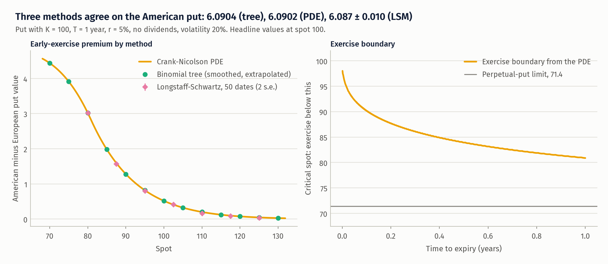
The left panel plots the early-exercise premium, which is a harder test than the price itself: the tree and the PDE are indistinguishable (0.0002 apart at the money) and the LSM points sit on the curve within two standard errors. LSM prices a Bermudan option with 50 dates and is biased low by its suboptimal stopping rule, so I compare it with a tree restricted to the same 50 dates; it is 0.85 standard errors above that tree. The right panel is the exercise boundary from the PDE, which starts at the strike and falls towards the perpetual-put limit \(K\gamma/(1+\gamma)\) with \(\gamma = 2r/\sigma^2\).
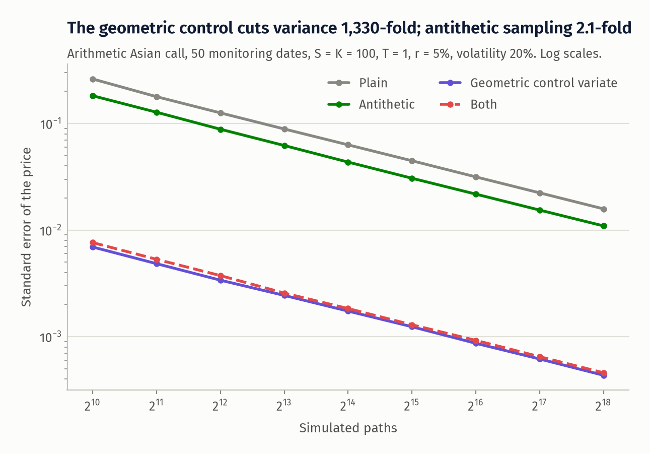
All four estimators converge at the \(n^{-1/2}\) rate; variance reduction only moves the constant. The geometric control variate cuts the variance by a factor of 1,330, because the two payoffs are almost perfectly correlated (\(\hat\beta = 1.035\)). Antithetic sampling gives a factor of 2.1. Combining the two gives 1,186, slightly worse than the control alone: once the control has removed the part of the payoff that is nearly linear in the path, there is little odd-symmetric variance left for the antithetic pair to cancel.
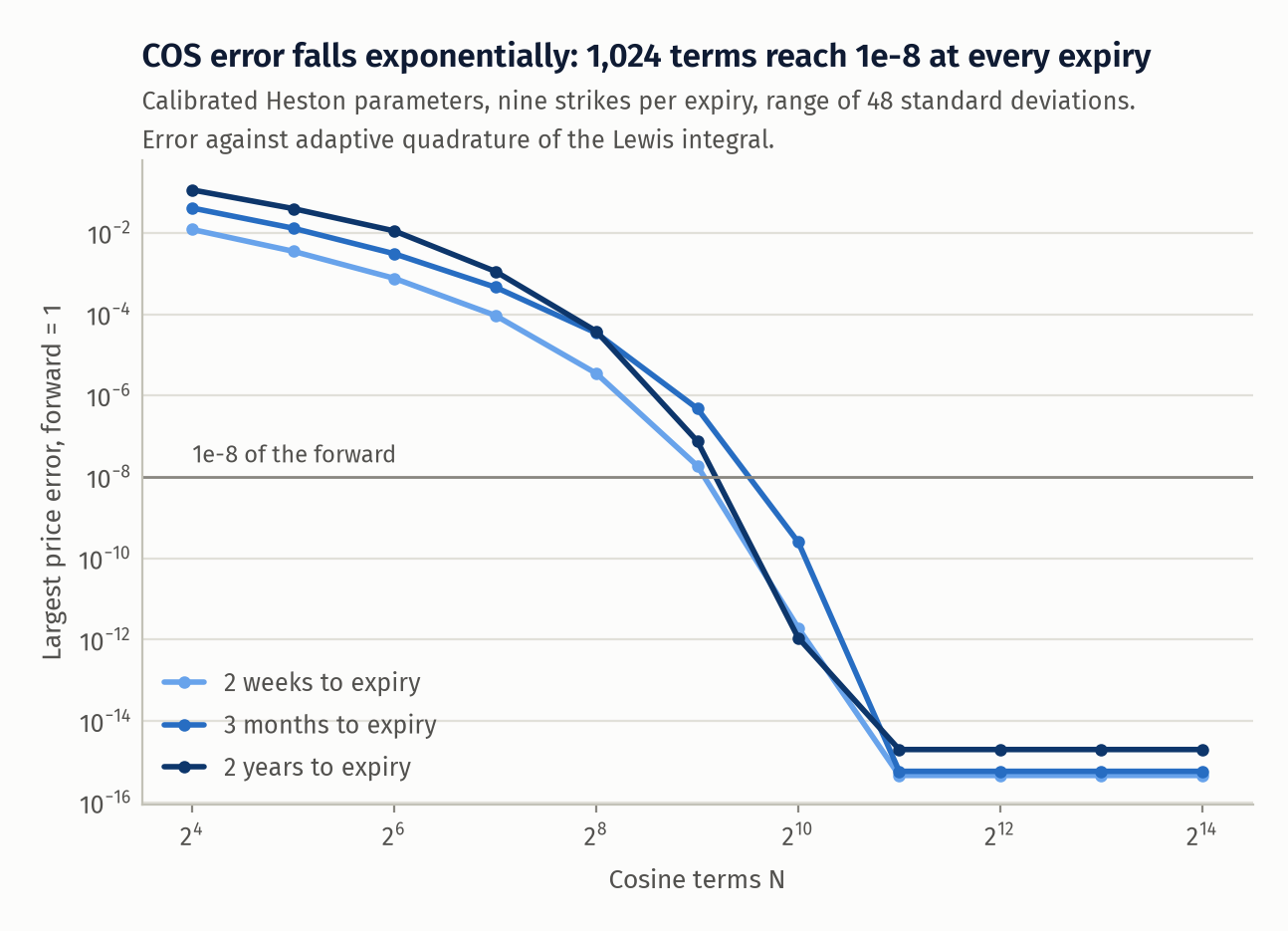
At the calibrated parameters the COS error against quadrature falls exponentially at all three maturities until it reaches the rounding floor. The adaptive rule picks 1,024 terms for the two-week expiry.
Handling American exercise
| Expiry | Contract | Mid | Early-exercise premium | Share of mid | Shift in implied vol |
|---|---|---|---|---|---|
| 1 month | 715 put | 3.96 | 0.03 | 0.8% | 0.06 vol points |
| 3 months | 691 put | 6.93 | 0.07 | 1.1% | 0.09 |
| 1 year | 640 put | 19.29 | 0.89 | 4.6% | 0.46 |
| 2 years | 620 put | 26.70 | 2.32 | 8.7% | 0.90 |
| any | out-of-the-money calls | 0.00 | 0.0% | 0.00 |
The premium on out-of-the-money calls is zero to the cent, because the implied dividend yield is far below the rate. For puts it is negligible under three months and material beyond a year. The correction lowers implied vols by 0.03 vol points on average under one month and by 0.53 beyond one year, with a maximum of 4.2 points for long-dated puts struck between the spot and the forward, which are out of the money against the forward but in the money against the spot. The premium correction also moves the two-year forwards by up to 226 basis points relative to the uncorrected regression.
The pooled rate comes out at 5.64%, against a 13-week Treasury bill yield of 4.12% on the same day. I cannot verify that number against an independent funding curve, and it deserves suspicion. Three observations bear on it. First, with the pooled rate the implied dividend yield beyond one year is 1.33%, in line with SPY's trailing yield of 1.01% plus some growth, and the parity residual beyond one year is $0.07; imposing the bill rate instead raises that residual to $0.19. Second, expiries before the December ex-dividend date (which I take to be the third Friday, 18 December) should imply a zero yield but imply 1.05% on average, which says the short-end rate is about one point below the pooled rate: a flat rate is too crude. Third, the fixed point is weakly identified, since a higher trial rate removes a larger put premium and so lowers the fitted discount factors. What matters for the surface is the forward, which is far less sensitive than the rate: imposing the bill rate moves forwards by at most 30 basis points and implied vols by 0.15 vol points on average beyond one year (0.39 at most), and by less than 0.04 under three months.
The Heston fit
| \(v_0\) | \(\theta\) | \(\kappa\) | \(\xi\) | \(\rho\) | \(2\kappa\theta/\xi^2\) |
|---|---|---|---|---|---|
| 0.0272 | 0.0510 | 4.127 | 1.488 | -0.738 | 0.19 |
So spot volatility is \(\sqrt{v_0} = 16.5\%\), long-run volatility is \(\sqrt{\theta} = 22.6\%\), and variance mean-reverts with a half-life of about two months. All five polished starts converge to the same point and no parameter is at a bound. The Feller condition fails badly, so the fitted variance process spends time at zero; that is typical of equity-index calibrations and is one reason the simulation check uses the QE scheme.
| Expiry bucket | Quotes | Heston RMSE | SVI RMSE | Heston mean error: far put wing | near the money | call wing |
|---|---|---|---|---|---|---|
| under 1 month | 455 | 0.89 | 0.13 | -0.56 | +0.26 | +0.56 |
| 1 to 3 months | 573 | 0.52 | 0.07 | -0.16 | -0.51 | +0.22 |
| 3 to 12 months | 661 | 0.43 | 0.28 | -0.26 | -0.34 | 0.00 |
| over 1 year | 606 | 0.55 | 0.15 | -0.58 | +0.58 | -0.15 |
| all | 2,295 | 0.60 | 0.18 |
All numbers are in vol points; the wings are \(k/(0.2\sqrt{T}) < -1.5\) and \(> 0.75\), near the money is within \(\pm 0.5\).
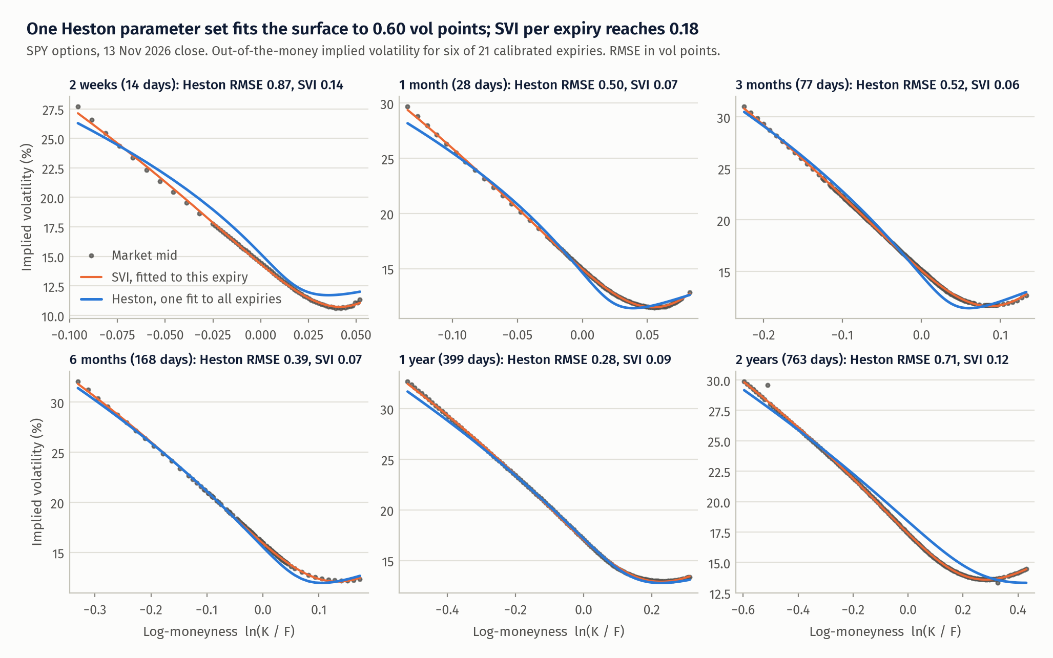
From one month to one year Heston follows the smile closely. At two weeks it bows above the market through the middle of the put side and falls below it in the far wing; at two years it is too high near the money and too flat on the call side.
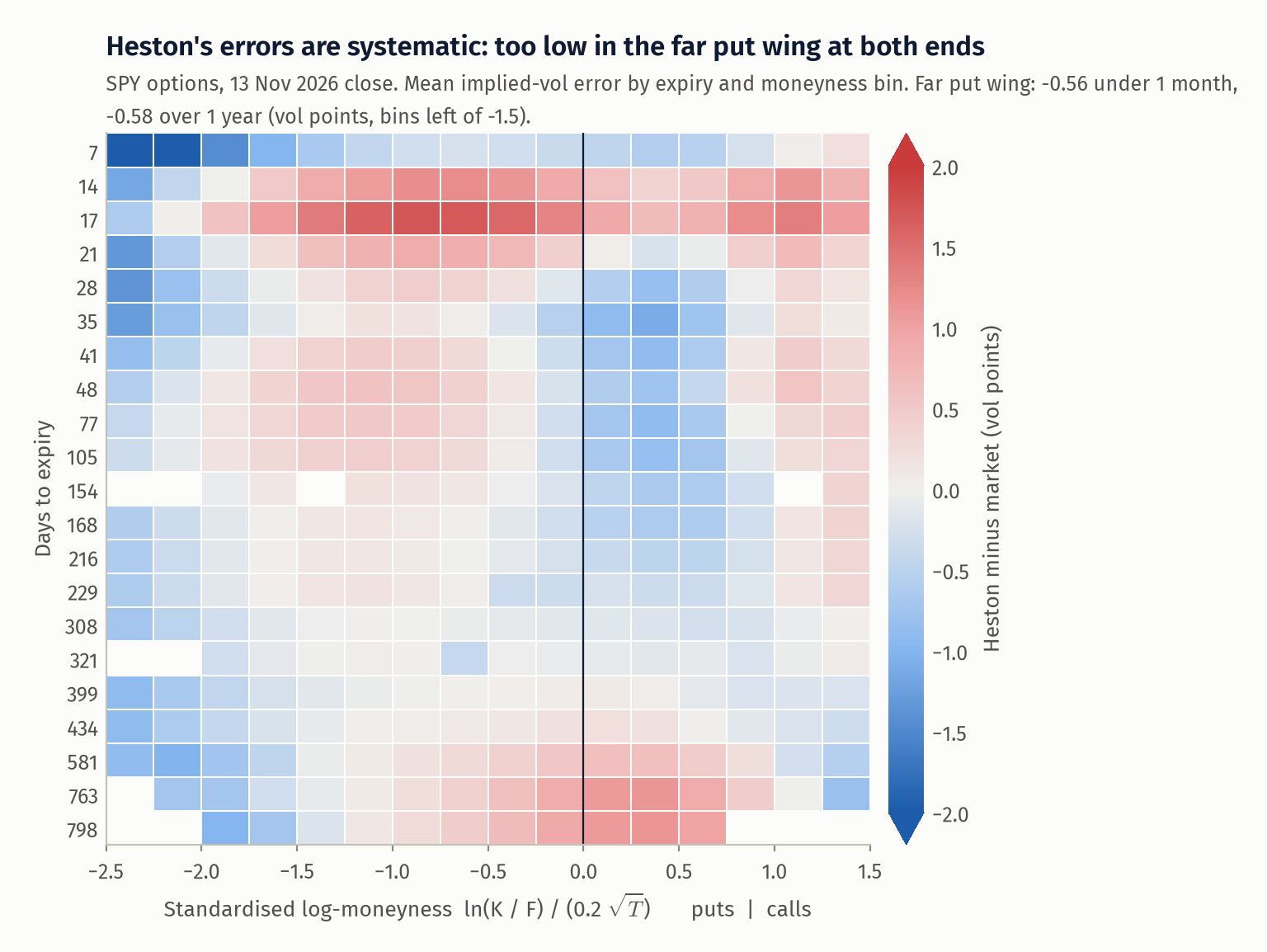
The errors are organised, not random. The far put wing is too low at almost every expiry, the band just below the money is too high for the shortest expiries, and at the long end the sign pattern flips around the money.
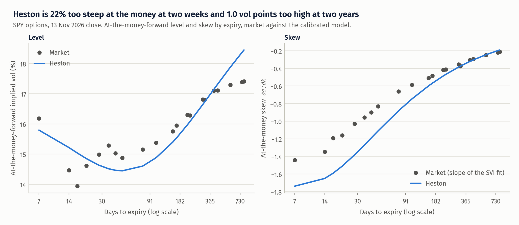
I expected to find that Heston cannot produce enough short-dated skew. That is not quite what this snapshot shows. At the money the calibrated model is steeper than the market: the two-week skew \(\partial\sigma/\partial k\) is -1.65 in the model against -1.35 in the market, 22% too steep, and the gap closes by one year (-0.32 against -0.31). What Heston cannot produce is the shape. The market's two-week smile is close to a straight line from \(k = -0.10\) to \(k = +0.03\), while the Heston smile is concave on the put side and flattens in the wing. With a small-time at-the-money skew of roughly \(\rho\xi/(4\sqrt{v_0})\), the only way for the model to lift the far put wing is a large \(\xi\), and the optimiser pays for that with too much slope at the money and call-side vols that are too high. On the level, one mean-reversion speed cannot match both ends of the term structure: the model is 1.0 vol point too high at two years (18.4% against 17.4%), and it cannot follow the uneven first three weeks, where market at-the-money vol runs from 13.9% to 16.2%.
Explore the smile
The pricers below are JavaScript ports of the Python ones, checked against them by an automated script. The first shows the calibration result and lets you break it.
What this does not show
- One snapshot. I have not tested whether the parameters are stable from day to day, whether the model hedges well, or how it prices anything out of sample. A good fit on one date says little about dynamics.
- Data quality. Yahoo closing quotes are not synchronised with each other or with the underlying. The SPY close was 754.37; the spot implied by the nearest expiry's forward is 752.39, 26 basis points lower. I use the option-implied spot throughout so that the chain is consistent with itself.
- The pooled rate is unverified, as discussed above, and is a single flat number where the data ask for a term structure.
- Long-dated put vols depend on a model. The early-exercise premium comes from a Black-Scholes tree at each option's own implied vol with a continuous dividend yield. SPY pays discrete quarterly dividends and has a smile. The correction reaches 4.2 vol points for some long-dated puts, so the long-end put side of the surface is partly an output of that tree. European SPX options would avoid the problem entirely.
- Mid prices and equal weights. The fit is to mids with no weighting by spread or vega. A desk would weight by vega over spread and would care about bid-ask violations more than RMSE.
- SVI is unconstrained. I fit each slice freely and did not check butterfly or calendar arbitrage, so the SVI benchmark may not be an arbitrage-free surface.
- Model scope. No jumps, no rough or multi-factor volatility, no time-dependent parameters. Any of these would improve the short end, which is where single-factor Heston is known to struggle.
- Longstaff-Schwartz is run with 50 exercise dates and a cubic basis, so it prices a Bermudan approximation with a low bias.
What I would do next
- Repeat the calibration on European SPX options, where forwards come from parity with no premium correction, and see how much of the long-end misfit survives.
- Calibrate daily over a year and look at parameter stability, then test the delta and vega hedges implied by the model against realised changes.
- Add a second variance factor or jumps (Bates) and measure the improvement under one month against the extra parameters.
- Replace the flat rate with a rate per expiry bucket and model the dividends as discrete cash amounts in the tree.
- Weight residuals by vega over spread and report the share of quotes inside the bid-ask as the main metric.
References
- Albrecher, H., Mayer, P., Schoutens, W. and Tistaert, J. (2007). The little Heston trap. Wilmott Magazine, January, 83-92.
- Andersen, L. (2008). Simple and efficient simulation of the Heston stochastic volatility model. Journal of Computational Finance 11(3), 1-42.
- Black, F. (1976). The pricing of commodity contracts. Journal of Financial Economics 3, 167-179.
- Black, F. and Scholes, M. (1973). The pricing of options and corporate liabilities. Journal of Political Economy 81(3), 637-654.
- Broadie, M. and Detemple, J. (1996). American option valuation: new bounds, approximations, and a comparison of existing methods. Review of Financial Studies 9(4), 1211-1250.
- Cox, J., Ross, S. and Rubinstein, M. (1979). Option pricing: a simplified approach. Journal of Financial Economics 7(3), 229-263.
- Fang, F. and Oosterlee, C. W. (2008). A novel pricing method for European options based on Fourier-cosine series expansions. SIAM Journal on Scientific Computing 31(2), 826-848.
- Gatheral, J. and Jacquier, A. (2014). Arbitrage-free SVI volatility surfaces. Quantitative Finance 14(1), 59-71.
- Glasserman, P. (2004). Monte Carlo Methods in Financial Engineering. Springer.
- Heston, S. L. (1993). A closed-form solution for options with stochastic volatility with applications to bond and currency options. Review of Financial Studies 6(2), 327-343.
- Kemna, A. G. Z. and Vorst, A. C. F. (1990). A pricing method for options based on average asset values. Journal of Banking and Finance 14(1), 113-129.
- Lewis, A. L. (2001). A simple option formula for general jump-diffusion and other exponential Lévy processes. Working paper.
- Longstaff, F. A. and Schwartz, E. S. (2001). Valuing American options by simulation: a simple least-squares approach. Review of Financial Studies 14(1), 113-147.
- Manaster, S. and Koehler, G. (1982). The calculation of implied variances from the Black-Scholes model: a note. Journal of Finance 37(1), 227-230.
- Merton, R. C. (1973). Theory of rational option pricing. Bell Journal of Economics and Management Science 4(1), 141-183.
- Rannacher, R. (1984). Finite element solution of diffusion problems with irregular data. Numerische Mathematik 43, 309-327.