Research / Forecasting
Does machine learning beat a three-parameter model at forecasting volatility?
Abstract. I compare eleven volatility forecasts, from a random walk to pooled gradient boosting, on 30 liquid US-listed ETFs and stocks, walk-forward from 2010 to November 2026 (4,242 one-day forecasts per asset). Against the standard HAR regression, LightGBM lowers the pooled QLIKE loss by 9.7% one day ahead and 10.8% five days ahead, with a significant Diebold-Mariano win on 21 and 13 of 30 assets, and no gain at 22 days (QLIKE ratio 1.014). The same HAR estimated in logs gets 7.0%, 11.8% and 9.3%, sits in the 90% model confidence set at all three horizons, and beats LightGBM on 14 of 30 assets at 22 days while losing on 7 at one day. In mean squared error the boosted model is no better than HAR (ratio 1.000 one day ahead). When each forecast is used to target 10% volatility on SPY, every sensible model lands between 8.8% and 10.8% realised volatility with a net Sharpe ratio of 0.72 to 0.75, against 0.76 for buy and hold.
So the answer in this sample is: a little, at short horizons, in one loss function, and a change of functional form in the linear model recovers most of it.
- Question
- Is a pooled gradient-boosting model a better volatility forecaster than the HAR regression?
- Data
- 30 liquid US-listed ETFs and stocks, daily bars, 2005 to November 2026; 4,242 out-of-sample days per asset
- Methods
- Range-based variance estimators, HAR, GARCH, LightGBM, QLIKE loss, Diebold-Mariano tests, model confidence set
- Verification
- 26 tests, including proof that no feature or forecast uses future data
The question
Volatility is the one input to position sizing, option pricing and risk limits that is forecastable. The benchmark that has been hard to beat for fifteen years is the HAR model of Corsi (2009): a linear regression of future variance on its averages over the last day, week and month. It has three slope parameters.
A machine learning engineer's instinct is that a flexible model with more features should do better. The published evidence says the gains are modest and come mostly from pooling across assets and adding implied volatility. I wanted to measure this myself under conditions I would defend in a review: strong simple baselines, strictly time-ordered validation, a loss function that is valid for a noisy target, significance tests, and no choices made after seeing test results.
The mathematics
Measuring variance from daily bars
True variance is not observable. Without intraday data I estimate each day's variance from its open, high, low and close. With previous close \(C'\), write \(o=\ln(O/C')\), \(u=\ln(H/O)\), \(d=\ln(L/O)\), \(c=\ln(C/O)\). For a driftless Brownian motion with open-to-close variance \(\sigma^2\):
| Estimator | Formula | \(\mathrm{Var}/\sigma^4\) | Efficiency |
|---|---|---|---|
| Squared return | \(c^2\) | 2.000 | 1.0 |
| Parkinson (1980) | \((u-d)^2/(4\ln 2)\) | 0.407 | 4.9 |
| Rogers-Satchell (1991) | \(u(u-c)+d(d-c)\) | 0.331 | 6.0 |
| Garman-Klass (1980) | \(\tfrac12(u-d)^2-(2\ln 2-1)c^2\) | 0.270 | 7.4 |
All four are unbiased; efficiency is \(\mathrm{Var}(c^2)/\mathrm{Var}(\text{estimator})\). The Parkinson value is exact, from \(E[(u-d)^2]=4\ln 2\,\sigma^2\) and \(E[(u-d)^4]=9\zeta(3)\sigma^4\). A simulation with exact (Brownian-bridge) highs and lows reproduces the other two: 4.92, 6.01 and 7.42. Rogers-Satchell stays unbiased with drift; Parkinson and Garman-Klass do not, which is irrelevant at a one-day horizon. Yang and Zhang (2000) combine overnight variance, open-to-close variance and Rogers-Satchell into an estimator that is unbiased with drift and opening jumps, but it needs a window of days, so it cannot be a one-day target. All four are implemented in estimators.py.
The target is
$$RV_t = o_t^2 + GK_t ,$$the squared overnight return plus Garman-Klass for the trading session, and for horizon \(h\)
$$y_t^{(h)} = \frac1h\sum_{j=1}^{h} RV_{t+j}, \qquad h\in\{1,5,22\}.$$I chose Garman-Klass over Rogers-Satchell for two reasons: it is the more efficient of the two, and it is strictly positive whenever the bar has a range (because \((u-d)^2\ge c^2\) and \(\tfrac12 > 2\ln2-1\)), whereas Rogers-Satchell is exactly zero on any day that opens at the low and closes at the high. In my data the proxy is positive on every one of 165,060 bars. Rogers-Satchell would have produced zeros, which break both the log models and QLIKE.
Why a noisy target does not invalidate the comparison
\(RV_t\) is a noisy measurement of the true conditional variance \(\sigma_t^2\). Patton (2011) asks when ranking forecasts by their average loss against a proxy \(\hat\sigma^2\) gives the same ranking as against \(\sigma^2\), and shows that this holds for a specific family of loss functions provided the proxy is conditionally unbiased, \(E_{t-1}[\hat\sigma_t^2]=\sigma_t^2\). The family contains MSE and
$$\mathrm{QLIKE}(y,f)=\frac{y}{f}-\ln\frac{y}{f}-1 .$$The reason is short. The part of QLIKE that depends on the forecast is \(\ln f + y/f\), which is linear in \(y\). Taking conditional expectations replaces \(y\) by \(\sigma^2\), so the expected loss against the proxy equals the expected loss against the truth plus a term that does not involve \(f\). For MSE, \(E[(\hat\sigma^2-f)^2]=E[(\sigma^2-f)^2]+E[(\hat\sigma^2-\sigma^2)^2]\) because the cross term vanishes. Noise adds a constant to every model's loss; it lowers the power of tests but does not bias the ranking. Losses that are not linear in \(y\) in this way fail: mean absolute error on squared returns is minimised by the conditional median of \(\sigma^2\chi^2_1\), which is \(0.455\,\sigma^2\), so it rewards a forecast that is 55% too low. tests/test_evaluation.py demonstrates all three statements on simulated GARCH data.
I report both losses and treat QLIKE as primary. QLIKE depends only on the ratio \(y/f\), so it weights a calm bond ETF and a stock in a crash equally, and it penalises under-prediction more than over-prediction, which is the right asymmetry for risk. MSE in a pooled sample is decided by a handful of crisis days.
QLIKE is also half the unit deviance of a gamma distribution. LightGBM's built-in gamma objective therefore trains the booster directly on the loss it is judged by.
Two caveats on unbiasedness. Range estimators assume continuous monitoring and no bid-ask bounce; discrete trading biases them down (9% with 390 observations a day in simulation, right panel of the last figure), bounce biases them up. Across my 30 assets the ratio of mean \(RV\) to mean squared close-to-close return runs from 0.88 to 1.32 with median 1.04. A constant multiplicative bias per asset does not change rankings between models fit to the same proxy, but it would penalise models fit to returns, so I rescale those (below). As a check I also re-rank all one-day forecasts against squared returns, which are unbiased without any diffusion assumption: the rank correlation of the eleven models' losses under the two proxies is 0.99.
Models
All forecasts are of \(y_t^{(h)}\), made at the close of day \(t\).
- Random walk: \(RV_t\). 22-day mean: \(RV^{(22)}_t\), the "historical volatility" on any terminal.
- EWMA (RiskMetrics): \(s^2_{t+1}=\lambda s^2_t+(1-\lambda)r_t^2\), \(\lambda=0.94\), flat across horizons.
- GARCH(1,1) and GJR-GARCH on close-to-close returns, zero mean, Gaussian quasi-likelihood: \(s^2_{t+1}=\omega+(\alpha+\gamma\,1[r_t<0])r_t^2+\beta s^2_t\). With \(p=\alpha+\gamma/2+\beta\) and \(\bar v=\omega/(1-p)\), the average expected variance over \(h\) days is
- HAR (Corsi 2009), per asset, by OLS: \(y^{(h)}_t=\beta_0+\beta_d RV_t+\beta_w RV^{(5)}_t+\beta_m RV^{(22)}_t+\varepsilon_t\), where \(RV^{(k)}_t\) is the mean of the last \(k\) days. This is the benchmark. It nests the two naive forecasts in (1). HAR (log): the same regression with every variable in logs. \(\exp\) of the fitted value estimates the conditional median, not the mean; under normal errors the mean is \(\exp(\text{fit}+s^2/2)\). I use Duan's (1983) smearing estimate, which multiplies by the sample mean of \(\exp(\text{residual})\) and assumes no distribution.
- HAR-X: HAR in levels plus \(r_t^2\,1[r_t<0]\) (leverage) and \(\mathrm{VIX}_t^2/252\).
- Panel HAR: one set of coefficients for all assets, on variance divided by each asset's own expanding mean \(s_{i,t}\) (known at \(t\)).
- LightGBM, pooled across assets, target \(y^{(h)}_{i,t}/s_{i,t}\), gamma objective, 17 features: variance averaged over 1, 5, 22 and 66 days; downside variance \(r^2 1[r<0]\) over 1, 5 and 22 days; standardised returns over 1, 5 and 22 days; VIX level, 1-day and 5-day log changes, VIX/VIX3M, and VIX variance relative to the asset's own; the asset's long-run volatility; day of week.
- Average of HAR and LightGBM.
EWMA and the GARCH models forecast squared returns, not \(RV\). Each is multiplied by the ratio of mean \(RV\) to mean \(r^2\) in that asset's training window, so the comparison is about dynamics and not about the level of the proxy.
Tests of forecast accuracy
For loss differential \(d_t=L_{A,t}-L_{B,t}\) the Diebold-Mariano (1995) statistic is \(\bar d/\sqrt{\widehat{\mathrm{LRV}}(d)/n}\). I use a Newey-West variance with bandwidth \(\max(\lfloor 4(n/100)^{2/9}\rfloor,\,2(h-1))\), wide enough to cover the MA(\(h-1\)) structure that overlapping targets induce, apply the Harvey-Leybourne-Newbold (1997) factor \(\sqrt{(n+1-2h+h(h-1)/n)/n}\) and compare with \(t_{n-1}\). The Model Confidence Set of Hansen, Lunde and Nason (2011) is the set of models that contains the best one with 90% confidence; I compute it on the cross-sectional mean QLIKE per day with a stationary bootstrap (block length 22, 1,000 replications, seed 0).
Method
Data. Daily bars from Yahoo Finance, 3 January 2005 to 13 November 2026, 5,502 days, for 18 ETFs (SPY, QQQ, IWM, DIA, EFA, EEM, TLT, IEF, LQD, GLD and eight sector funds) and 12 large stocks (AAPL, MSFT, AMZN, GOOGL, JPM, XOM, JNJ, WMT, PG, KO, INTC, CSCO), plus ^VIX, ^VIX3M and ^IRX. Yahoo's raw OHLC is adjusted for splits but not dividends. I multiply all four prices of each day by Adj Close / Close, which leaves within-day ratios untouched and removes the ex-dividend drop from the overnight return. No bar needed repair (no missing values, no high below the close, no zero range). I do not winsorise the target: the flash-crash prints of 6 May 2010 are real trades. VIX9D starts in 2011 and is not used; VIX3M starts in July 2006 and is missing (handled natively by LightGBM) before that.
Validation. Expanding window, every model refitted once a year, test years 2010 to 2026. For test year \(Y\) let \(T\) be the last trading day before it. A training row is an origin \(s\) with \(s+h\le T\), so for \(h>1\) the last \(h-1\) origins are purged and no training target overlaps the test period. Features at \(t\) use data dated \(t\) or earlier. Both properties are tested: replacing all data after a date leaves every feature and every model's forecast up to that date bit-for-bit unchanged.
LightGBM settings. Fixed: learning rate 0.05, feature fraction 0.8, L2 penalty 1, 63 bins, seed 0. Chosen at each refit from data inside the training window only: tree size among (4, 8, 16) leaves and the number of rounds (early stopping, at most 500), on a validation block made of the last 504 days of the training window, separated from the fitting block by \(h\) days. The model is then refitted on the whole training window. Across the 17 refits the median number of rounds was 173, 125 and 119 for the three horizons.
Fixed before any test result: the universe, the target, \(\lambda=0.94\), the HAR lags, the feature list, the hyperparameter grid, the DM bandwidth rule, the 5% and 10% test sizes, the stress definition (top decile of VIX at the forecast origin), the volatility target (10%), leverage cap (2) and trading cost (1 bp). Every forecast is floored at the smallest target in that asset's training window. I did not revisit any of these after seeing results, including the ones that turned out badly (HAR-X, the panel HAR).
Results
Accuracy
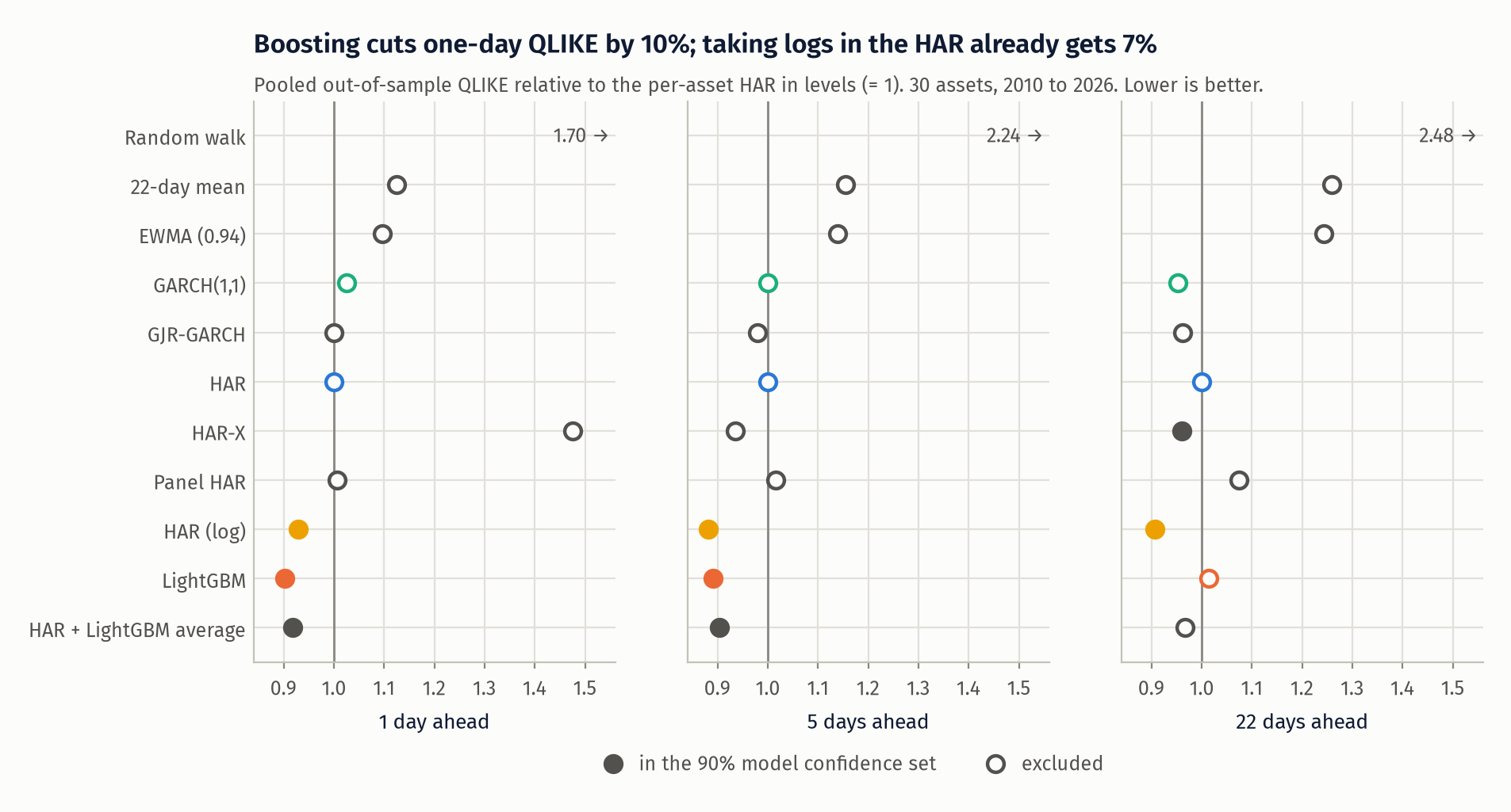
Pooled out-of-sample QLIKE and MSE relative to HAR (lower is better), and the number of assets out of 30 with a significant DM win / loss against HAR in QLIKE. An asterisk marks membership of the 90% model confidence set.
| Model | QLIKE h=1 | h=5 | h=22 | DM wins/losses h=1 | h=5 | h=22 | MSE h=1 | h=5 | h=22 |
|---|---|---|---|---|---|---|---|---|---|
| Random walk | 1.700 | 2.244 | 2.483 | 0 / 29 | 0 / 30 | 0 / 29 | 1.734 | 3.446 | 5.746 |
| 22-day mean | 1.124 | 1.154 | 1.259 | 1 / 23 | 1 / 18 | 0 / 10 | 1.056 | 1.167 | 1.348 |
| EWMA (0.94) | 1.097 | 1.138 | 1.242 | 1 / 21 | 1 / 18 | 0 / 8 | 1.016 | 1.055 | 1.128 |
| GARCH(1,1) | 1.025 | 0.999 | 0.953 | 3 / 16 | 2 / 5 | 7 / 1 | 0.986 | 0.970 | 0.936 |
| GJR-GARCH | 1.001 | 0.980 | 0.962 | 4 / 9 | 5 / 5 | 3 / 1 | 0.977 | 0.952 | 0.962 |
| HAR | 1.000 | 1.000 | 1.000 | 1.000 | 1.000 | 1.000 | |||
| HAR-X | 1.475 | 0.936 | 0.960* | 7 / 15 | 19 / 3 | 17 / 2 | 0.983 | 0.933 | 0.963 |
| Panel HAR | 1.006 | 1.015 | 1.074 | 8 / 17 | 5 / 17 | 1 / 20 | 1.027 | 1.069 | 1.133 |
| HAR (log) | 0.930* | 0.882* | 0.907* | 24 / 0 | 26 / 0 | 15 / 0 | 0.974 | 0.939 | 0.883 |
| LightGBM | 0.903* | 0.892* | 1.014 | 21 / 1 | 13 / 0 | 2 / 1 | 1.000 | 1.014 | 0.962 |
| HAR + LightGBM average | 0.917* | 0.904* | 0.967 | 29 / 0 | 29 / 0 | 8 / 0 | 0.977 | 0.957 | 0.911 |
What this shows:
- The ML gain is real at one and five days and absent at 22. LightGBM has the lowest one-day QLIKE (0.903) and is within a point of the best at five days. At 22 days it is level with HAR and 11.7% worse than the log HAR, which beats it significantly on 14 assets and loses on none.
- Most of the gain is functional form, not machine learning. Taking logs in a three-regressor OLS gets 7.0% of the 9.7% at one day and more than LightGBM at the other two horizons. Head to head in QLIKE, LightGBM against the log HAR is 0.971 at one day (7 significant wins, 1 loss), 1.011 at five days (2 and 3) and 1.117 at 22 days (0 and 14). The model confidence set cannot separate them at one and five days. Variance is close to lognormal, a levels regression is dominated by its largest observations, and both the log transform and the gamma objective fix that.
- In MSE there is nothing. LightGBM's MSE ratio is 1.000, 1.014 and 0.962, and its median out-of-sample \(R^2\) against the expanding mean (0.156 at one day) is below HAR's (0.190). It was trained on QLIKE and it is better in QLIKE. A reader who only looks at \(R^2\) would conclude ML lost.
- Averaging is the most reliable improvement. The equal-weight average of HAR and LightGBM is never the best model but beats HAR significantly on 29 of 30 assets at one and five days and never loses.
- GARCH is not embarrassed. Once its level is matched to the proxy, GARCH(1,1) is within 2.5% of HAR at one day and 4.7% better at 22 days, where its mean reversion to a long-run level helps. The simple filters without mean reversion (EWMA, rolling mean) lose 10% to 26%.
- Two of my ex-ante choices performed badly. HAR-X in levels has a pooled one-day QLIKE of 1.475, although its median per-asset ratio is 1.082 and it wins at 5 and 22 days: the linear leverage and VIX terms occasionally push a forecast close to the floor, and QLIKE punishes a forecast that is far too low very heavily. The panel HAR is worse than per-asset HAR at every horizon, so pooling by itself is not what helps the boosted model.
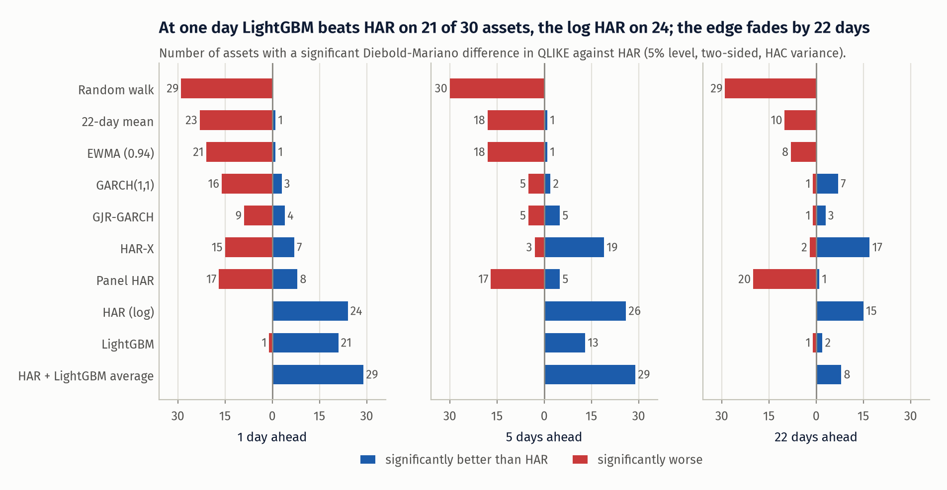
The asset-level tests agree with the pooled numbers. With 30 tests at the 5% level, one or two rejections in either direction are what chance alone produces.
Where the boosted model's gain comes from
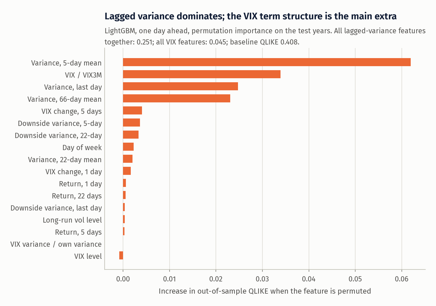
Permuting a feature across the test rows and measuring the increase in QLIKE (baseline 0.408 on scaled variance): all four lagged-variance features together cost 0.251, all VIX features 0.045, returns and downside variance 0.014, day of week 0.003, the long-run volatility level 0.0004. Among single features the 5-day variance is first (0.062) and the VIX term-structure slope, VIX/VIX3M, is second (0.034), ahead of yesterday's variance. The VIX level itself adds nothing once the asset's own variance is known. The boosted model is, in effect, a nonlinear HAR with one piece of forward-looking information from the options market. Correlated features share importance under permutation, so the single-feature numbers understate each lag; the grouped numbers do not have this problem.
Regimes
One-day and 22-day QLIKE relative to HAR on calm days and on stressed days (VIX at the forecast origin in its top decile, above 26.7; 426 of 4,242 days), and median out-of-sample \(R^2\):
| Model | calm h=1 | stressed h=1 | calm h=22 | stressed h=22 | OOS R² h=1 | h=5 | h=22 |
|---|---|---|---|---|---|---|---|
| GARCH(1,1) | 1.015 | 1.101 | 0.943 | 1.032 | 0.158 | 0.233 | 0.083 |
| HAR | 1.000 | 1.000 | 1.000 | 1.000 | 0.190 | 0.285 | 0.104 |
| HAR-X | 1.550 | 0.876 | 0.972 | 0.867 | 0.197 | 0.322 | 0.140 |
| HAR (log) | 0.923 | 0.982 | 0.904 | 0.929 | 0.206 | 0.299 | 0.192 |
| LightGBM | 0.905 | 0.885 | 0.993 | 1.176 | 0.156 | 0.201 | 0.129 |
| HAR + LightGBM average | 0.928 | 0.836 | 0.961 | 1.014 | 0.205 | 0.290 | 0.172 |
LightGBM's one-day advantage holds in both regimes, but at 22 days it is 17.6% worse than HAR when VIX is high. By calendar year its worst year at every horizon is 2020 or another stress year (QLIKE ratio 1.09 at one day and 1.24 at 22 days in 2020; 1.59 at 22 days in 2011). HAR-X is the mirror image: the VIX term earns its keep in stress and hurts in calm markets.
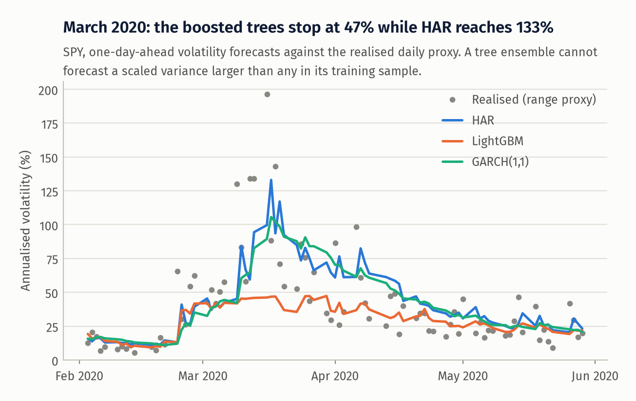
The figure shows why. A tree predicts the average of the training targets in a leaf, so it cannot forecast a scaled variance larger than any it has seen. In March 2020 the HAR and GARCH forecasts for SPY follow realised volatility above 100% while LightGBM stops below 50%. A linear model extrapolates; a tree ensemble saturates. This is the strongest practical argument for the average, and for not using trees alone in a risk system.
Economic value: volatility targeting on SPY
Each day the weight is \(w_t=\min(10\%/\hat\sigma_t,\,2)\) from the one-day forecast made at the close of day \(t\), traded at the close of \(t+1\) and held over day \(t+2\), financed at the 13-week bill rate, with 1 bp cost per unit traded (Moreira and Muir 2017 scale by inverse variance monthly; this is the daily analogue).
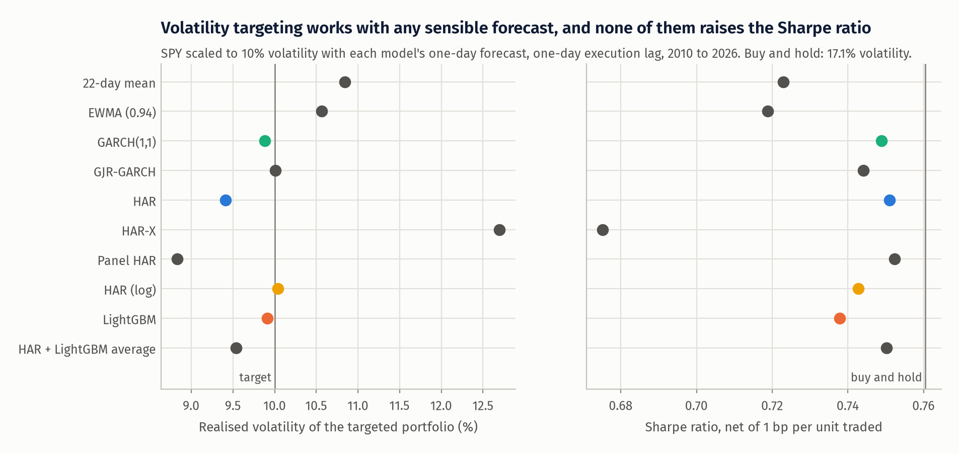
| Forecast | Realised vol | Vol of 63-day vol | Sharpe (net) | Max drawdown | Turnover / yr |
|---|---|---|---|---|---|
| Buy and hold | 17.1% | 7.9% | 0.76 | -33.8% | 0.0 |
| Random walk | 12.9% | 1.6% | 0.72 | -23.6% | 92.1 |
| 22-day mean | 10.8% | 1.8% | 0.72 | -16.9% | 5.2 |
| EWMA (0.94) | 10.6% | 1.8% | 0.72 | -16.5% | 6.5 |
| GARCH(1,1) | 9.9% | 1.5% | 0.75 | -14.3% | 8.9 |
| GJR-GARCH | 10.0% | 1.4% | 0.74 | -14.4% | 10.2 |
| HAR | 9.4% | 1.4% | 0.75 | -17.2% | 16.7 |
| HAR-X | 12.7% | 3.2% | 0.68 | -28.2% | 37.2 |
| Panel HAR | 8.8% | 1.6% | 0.75 | -16.4% | 9.3 |
| HAR (log) | 10.0% | 1.3% | 0.74 | -16.9% | 21.3 |
| LightGBM | 9.9% | 1.5% | 0.74 | -17.0% | 21.1 |
| HAR + LightGBM average | 9.5% | 1.3% | 0.75 | -17.0% | 17.1 |
Volatility targeting does what it says: realised volatility falls from 17.1% to about 10%, its variability over time falls by a factor of five, and the maximum drawdown halves. But the choice of forecast barely matters. GARCH, GJR-GARCH, the log HAR and LightGBM all land within 0.1 points of the target; the Sharpe ratios of the nine sensible forecasts span 0.72 to 0.75 and none exceeds buy and hold (0.76). A 10% improvement in QLIKE is invisible to a portfolio manager in this application. The two forecasts with occasional very low values (random walk, HAR-X) are the ones that miss, because a forecast near zero means maximum leverage. One asset over 17 years is a single path, so differences of a few hundredths in Sharpe are not distinguishable from noise.
Range estimators
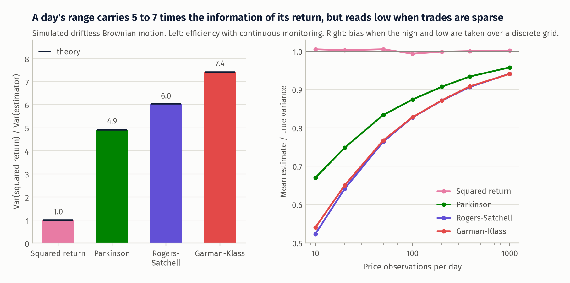
Simulated efficiencies match theory (left). The right panel is the caveat: with highs and lows observed on a discrete grid, range estimators are biased down, by about 9% at 390 observations a day. For the names in this study, which trade thousands of times a day, the ratio of the proxy to squared returns is close to one (median 1.04), but I would not use this target for illiquid assets without correcting for it.
What this does not show
- The target is a proxy. Rankings in QLIKE and MSE are valid under conditional unbiasedness; the size of the losses, the \(R^2\) values and the power of the tests are all degraded by noise. With 5-minute realised variance the gaps between models would be estimated more sharply and might change in size.
- The universe was chosen in 2026. All 30 names survived and stayed liquid for 22 years. Volatility forecasting is less exposed to survivorship than return prediction, but the sample contains no delisting or bankruptcy.
- Thirty assets are not thirty independent tests. Most are US equity exposures driven by one volatility factor, so "21 of 30" overstates the evidence. The model confidence set on pooled daily losses is the better guide.
- Diebold-Mariano with nested, re-estimated models. HAR-X and HAR are nested, for which the DM statistic is not asymptotically normal under the null of equal population accuracy. I read the tests in the Giacomini-White sense, as comparisons of forecasting methods including their estimation error.
- LightGBM was given one small grid. A larger search, monotonicity constraints, or a linear-plus-trees hybrid might do better, particularly on the extrapolation problem. I fixed the grid in advance and did not iterate on test results, so the numbers are an honest estimate for this specification, not an upper bound for ML.
- The VIX close is at 16:15 New York time, fifteen minutes after the stock close. Forecasts that use VIX have a small timing advantage.
- The volatility-targeting test assumes trading at the close at 1 bp, financing at the bill rate, and no constraint on daily rebalancing. It uses the one-day forecast for a position held one day later.
- Refitting is annual. Monthly refits would help every model a little; I did not test whether they would help some more than others.
What I would do next
- Replace the range proxy with 5-minute realised variance and realised semivariance for a subset of names, and check whether the log HAR result survives a cleaner target.
- Fix the extrapolation problem directly: boost the residual of the log HAR instead of the level, so the linear model handles the extremes and the trees handle the interactions.
- Add implied volatility per asset (not only VIX) and measure how much of the remaining gain is the variance risk premium.
- Evaluate on quantities closer to use: Value-at-Risk coverage, and option straddle P&L against implied volatility.
References
- Corsi, F. (2009). A simple approximate long-memory model of realized volatility. Journal of Financial Econometrics 7(2).
- Diebold, F. X. and Mariano, R. S. (1995). Comparing predictive accuracy. Journal of Business & Economic Statistics 13(3).
- Duan, N. (1983). Smearing estimate: a nonparametric retransformation method. Journal of the American Statistical Association 78.
- Garman, M. B. and Klass, M. J. (1980). On the estimation of security price volatilities from historical data. Journal of Business 53(1).
- Giacomini, R. and White, H. (2006). Tests of conditional predictive ability. Econometrica 74(6).
- Glosten, L. R., Jagannathan, R. and Runkle, D. E. (1993). On the relation between the expected value and the volatility of the nominal excess return on stocks. Journal of Finance 48(5).
- Hansen, P. R., Lunde, A. and Nason, J. M. (2011). The model confidence set. Econometrica 79(2).
- Harvey, D., Leybourne, S. and Newbold, P. (1997). Testing the equality of prediction mean squared errors. International Journal of Forecasting 13(2).
- Moreira, A. and Muir, T. (2017). Volatility-managed portfolios. Journal of Finance 72(4).
- Parkinson, M. (1980). The extreme value method for estimating the variance of the rate of return. Journal of Business 53(1).
- Patton, A. J. (2011). Volatility forecast comparison using imperfect volatility proxies. Journal of Econometrics 160(1).
- Rogers, L. C. G. and Satchell, S. E. (1991). Estimating variance from high, low and closing prices. Annals of Applied Probability 1(4).
- Yang, D. and Zhang, Q. (2000). Drift-independent volatility estimation based on high, low, open, and close prices. Journal of Business 73(3).